Path Tracer
A physically-based renderer that solves the rendering equation with Monte Carlo integration.
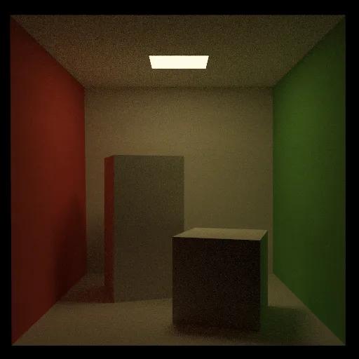
Overview
Photorealistic rendering boils down to solving the rendering equation: the light leaving any surface point equals the light it emits plus the integral, over every incoming direction, of incoming light weighted by the surface's BRDF (how the material scatters light) and the angle of incidence. It's an integral equation (the incoming light on the right side is itself outgoing light from other surfaces), so no closed-form solution exists for any interesting scene.
Essentially: outgoing light = emitted light + (for every incoming direction \(\omega_i\)) incoming light × material response × how directly the light hits the surface.
The core loop: Monte Carlo path tracing
Since there is no closed form solution, the integral has to be estimated numerically, and Monte Carlo integration is the one numerical method that doesn't care how high-dimensional or discontinuous the integrand is. Thus, you can sample random light paths, average them, and the average will eventually converges to the true image:
Each sample is divided by the probability of having chosen it, which keeps the estimate unbiased no matter how samples are drawn. Error shrinks with √N, which is why path-traced images start noisy and clean up as samples accumulate.
One sample of this estimator is a path, built one bounce at a time:
A ray into the scene
Shoot a camera ray through the pixel and find the closest surface it hits.
Sample a direction
Draw a random outgoing direction, multiply the path's running throughput by \(f_r \cos\theta / p(\omega)\), and continue from the hit point.
Russian roulette
The recursion has no natural end because light keeps bouncing. Kill the path probabilistically and reweight survivors, so paths stay finite without biasing the image.
Accumulate per pixel
Each completed path is one sample of the rendering equation; averaging hundreds per pixel converges to the solution.
Russian roulette: unbiased path termination
The rendering equation recurses forever because light keeps bouncing. Truncating paths at a fixed depth silently deletes all the energy those deeper bounces would have carried, which darkens the image: that's bias. Russian roulette terminates paths probabilistically instead. At each bounce, kill the path with probability \(q\); if it survives, divide its contribution by \(1-q\).
The survivors are boosted by exactly the factor needed to make up for the killed paths, so the expected value is untouched, so paths become finite while the estimator stays unbiased. The price is variance: the occasional long-surviving path carries a large weight. I keep \(q\) modest (around 0.3) and only start roulette after a few guaranteed bounces, so short paths (which carry most of the energy) are never gambled away.
Additional Steps to Speed Up Convergence
Sample where light matters
Diffuse bounces are drawn from a cosine-weighted distribution and glossy bounces from the Phong lobe around the mirror direction, so samples go where the integrand is largest.
Direct light sampling
At each bounce, the estimate splits into a direct part (pick a point on an area light and cast a shadow ray) and an indirect recursive part. Far more reliable than hoping a random bounce hits a small light.
Even pixel coverage
Sub-pixel samples are jittered within a grid rather than drawn purely at random, so samples cover each pixel evenly, which means less variance at no extra cost.
Event splitting: direct light sampling
A naive path tracer only finds light when a random bounce happens to hit an emitter. For small lights that almost never happens, so most paths contribute nothing and the image stays noisy. Event splitting fixes this by splitting the reflected radiance at every bounce into two estimators: a direct term, sampled by picking a point on a light source deliberately, and an indirect term, sampled by bouncing the path onward.
For the direct term, I sample a point \(y\) uniformly on an area light (\(p_A(y) = 1/A\)) and cast a shadow ray to test visibility. Because the sample is drawn over the light's surface rather than over directions, the integrand picks up a geometry term that converts between the two measures:
\(\cos\theta_x\) is the angle at the shaded point, \(\cos\theta_y\) the angle at the light (a light facing away contributes nothing), the squared distance gives the natural falloff, and \(V\) is the shadow ray's 0-or-1 visibility. To avoid counting the same energy twice, emission is ignored when an indirect bounce ray happens to land on a light, since that light was already accounted for by the direct term at the previous vertex. The exception is mirror and refractive bounces: their BRDF is a delta function that shadow rays can't sample, so emission is kept when following them.
Importance sampling: Lambertian and Phong
Monte Carlo variance comes from the mismatch between the integrand and the sampling distribution, and the ideal distribution is proportional to the integrand itself. Uniform hemisphere sampling wastes samples on grazing directions whose \(\cos\theta\) factor nearly zeroes them out.
Lambertian. The BRDF is constant (\(\rho/\pi\)), so the integrand is proportional to \(\cos\theta\) alone. I sample a cosine-weighted hemisphere (uniform point on the unit disk, projected up, which is Malley's method), whose pdf is exactly \(\cos\theta/\pi\). The weight then collapses:
Every bounce just multiplies the path throughput by the albedo, and the direction-dependent variance vanishes entirely.
Phong. The glossy lobe \(f_r \propto \cos^n\alpha\) concentrates around the mirror direction \(\omega_r\), and gets narrower as the exponent \(n\) grows. I sample directions around \(\omega_r\) with \(\cos\alpha = u_1^{1/(n+1)},\ \phi = 2\pi u_2\), giving \(p(\omega) = \frac{n+1}{2\pi}\cos^n\alpha\). The \(\cos^n\alpha\) in the pdf cancels the one in the BRDF, so a rough and a near-mirror surface converge equally fast instead of the tight lobe being missed by uniform samples.
Optics: refraction & depth of field
Two pieces of physical camera and material behavior, each with its own math.
Refraction: Snell, total internal reflection, Fresnel
At a dielectric boundary the transmitted direction follows Snell's law, \(\eta_1 \sin\theta_1 = \eta_2 \sin\theta_2\). Solving for the transmitted ray requires \(\sin^2\theta_t \le 1\); past the critical angle (glass-to-air at roughly 42°) there is no solution and all light reflects. This is total internal reflection, which is what makes the bottom of a glass object glitter.
Real dielectrics both reflect and refract, with the split governed by the Fresnel equations. I use Schlick's approximation:
Glass reflects ~4% head-on but almost 100% at grazing angles, which is why windows become mirrors at night when viewed obliquely. Rather than splitting every hit into two rays (which would branch the path tree exponentially), the path chooses: reflect with probability \(R\), refract with probability \(1-R\), each weighted by one over its probability. The Fresnel factor cancels against the weight, one ray continues, and the expected value is exactly the full split.
Depth of field: the thin-lens camera
A pinhole camera renders everything in perfect focus because every pixel sees through a single point. Real lenses have area, and that's where focus blur comes from. The thin-lens model adds two parameters: an aperture radius and a focal distance.
For each camera ray, first find the point \(P\) where the original pinhole ray crosses the focal plane. Then jitter the ray origin to a uniformly-sampled point on the aperture disk and aim the new ray at \(P\):
Every lens sample converges on \(P\), so geometry on the focal plane stays sharp no matter where on the aperture the ray started. Geometry off the plane is hit by rays from different lens points at different locations, and averaging those samples smears it into the circle of confusion, which is the bokeh, produced by the same Monte Carlo machinery. The aperture radius directly controls blur strength: shrink it to zero and the pinhole camera returns.
Results
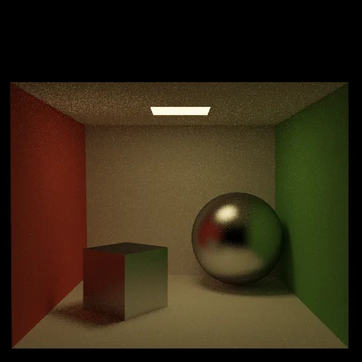
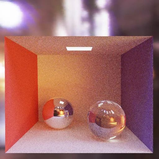
Features
Four BRDFs
Diffuse, glossy (Phong), ideal mirror, and refractive with Fresnel reflection via Schlick's approximation.
Soft shadows & caustics
Area light sampling and full indirect illumination with color bleeding.
Depth of field
Rays sampled across a camera aperture for physically-based focus falloff.
HDRI environments
Image-based environment lighting for natural outdoor illumination.